The purpose of this lab exercise is to familiarize students with multispectral imagery data sources used in Earth Observation applications, with the creation of colour composite images, and the use of the WhiteboxTools software package for analyzing these data.

The following materials, combined with your textbook, can be used as background materials and to help in answering the assignment questions.

• Baumann, P.R. 2010. Landsat Program

• NASA Landsat Science

• European Space Agency 2015. Sentinel-2 User Handbook

• Lindsay, J.B. 2019. The WhiteboxTools User Manual

IMPORTANT INFORMATION: This series of lab assignments will require manipulation, analysis, and visualization of several remotely sensed images. We will be separating the image analysis and data visualization components. For manipulating and analyizing remotely sensed data we will use the WhiteboxTools advanced geospatial analysis platform¹. For data visualization, these labs do not assume any particular remote sensing software. You are free to use whatever software you are familiar with for visualizing the imagery data in the labs, including ArcGIS, Whitebox Geospatial Analysis Tools¹ (Whitebox GAT), QGIS, or any other spatial anlysis software capable of displaying georeferenced imagery data.

¹ In this series of lab assignments, WhiteboxTools refers to the standalone geospatial analysis library, a collection of tools contained within a compiled binary executable command-line program and the associated Python scripts that are distributed alongside the binary file (e.g. whitebox_tools.py and wb_runner.py). Whitebox Geospatial Analysis Tools and Whitebox GAT refer to the GIS/RS software, which includes a user-interface (front-end), point-and-click tool interfaces, and cartographic data visualization capabilities. Importantly, WhiteboxTools and Whitebox GAT are related but separate projects.

The computers in the Geography Undergraduate Computing Lab (Hutt 236), have ArcGIS and Whitebox GAT installed (IDRISI may possibly be installed as well). If you are planning to carry out these assignments on your own computer, then it is important that you have WhiteboxTools installed along with one of the data visualization packages described above. WhiteboxTools is open-source, freely available, and works on Windows, MacOS, and Linux operating systems. It can be downloaded from here. Instructions on setting up and using WhiteboxTools can be found in the WhiteboxTools User Manual and you are advised to look over these materials before starting this lab.

In addition to the software, you will need to download the data associated with this lab exercise from the CourseLink page under the Lab 1 directory. The data for this laboratory is quite large and will require substantial data storage. It is advisable that you purchase a USB flash drive to dedicate to this course and to serve as the data backup. It is important that you backup all of the data for the lab assignment.

You will hand in a printed report summarizing the answer to each of the questions in the following exercise along with the necessary colour images. Notice that you will need to have paid your lab fee to have printing privileges in the Hutt building computer labs.

Satellite data can be acquired from a large number of locations, depending on application needs. Before you begin a project involving satellite imagery, you should consider several factors, including: the type of sensor you require (e.g. multispectral imagery, radar data, LiDAR data, etc.), the necessary spatial resolution, temporal factors (e.g. do you need an image for a specific date or time of year?), and your budget for acquiring imagery. There are many commercial providers of satellite imagery and the cost per km² of data can vary significantly. There also several sources of free satellite imagery, which, depending on your project constraints, may well be suitable.

The United States Geological Survey (USGS) are an excellent source of freely available satellite imagery data (2019 update: notice that the availability of these data may be affected by the current US government shutdown). The USGS are responsible for storing and disseminating many of the archived datasets from NASA satellites. There are two online data portals that the USGS currently operate to disseminate publically available imagery, including the Global Visualization Viewer (Glovis) and EarthExplorer. Visit the USGS Global Visualization Viewer web site at http://glovis.usgs.gov/

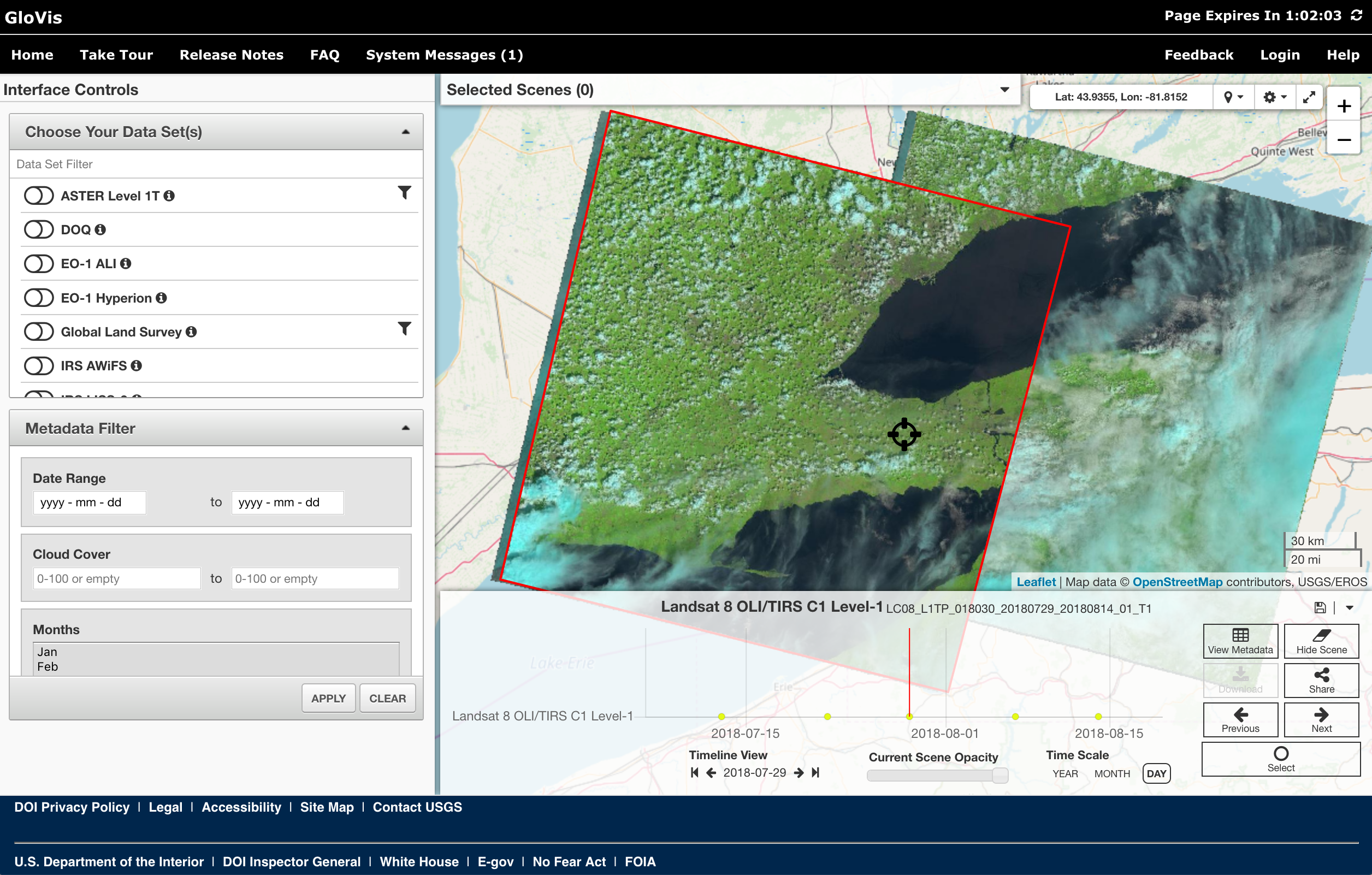
This is an excellent example of an online data warehouse for satellite imagery. Like many of these sites, you need to register before you are able to download the available data. We will not need to do this at the moment because even without registering, the site will allow users to examine historical and recently acquired images and assess their quality.

Examine each of the data sets that are available under the ‘Datasets menu. Not all of these data are available free-of-charge, and not every data set is available to users outside of the U.S., but many are. If you click on the ‘Data Descriptions’ link from within the sub-menu of any of the data sets, you will be able to see what data is available at no charge. The more interesting data sets include the ASTER, EO-1 ALI, EO-1 Hyperion (hyperspectral data), and the various available Landsat 5 TM, Landsat 7 ETM+, and Landsat 8 Operational Land Imager (OLI) collections. Select the Landsat 8 OLI option under the Landsat Archive menu. Now navigate to the Guelph area. Select the image tile that contains Guelph and most of the Greater Toronto Area. You will be able to view all of the images available in this collection corresponding with this location, scrolling through the timeline of acquisition dates at the bottom of the map. Notice that the image ID, scence cloud cover (CC) percentage, and date are given for each image.

The US-operated satellites are not the only source of remotely sensed imagery. Notably, the European Union also operate a number of earth observation satellites, including the Sentinel 1 and Sentinel 2 satellites which provide fine-resolution data (up to 10 m) freely. Like the Landsat program, the Sentinel program provides valuable data for many types of remote sensing applications.

1.1. What is meant by the row and path of a scene? What is the row and path of the scene that Guelph is contained within? (2 marks; hint, you should read the materials linked to in the introduction of the lab assignment.)

1.2. Provide the details (i.e. ID, scene cloud cover, quality, and date) of each of the images with the lowest cloud coverage in each of the available years (i.e. from 2013 to 2019). What was the cloud cover of the most recently acquired Landsat 8 OLI image (also provide the date the image was acquired) (7 marks).

1.3. What are the spectral resolutions, in μm, of the each of the Landsat 8 OLI sensor band data, i.e. what range of wavelengths does each band cover? (2 marks; again, you'll need to do a bit of digging in the assigned readings.)

1.4. What is a panchromatic band? How does its spectral resolution compare to that of the other multispectral bands within the Landsat 8 dataset? (2 mark)

1.5. Like the Landsat 8 OLI sensor, the Sentinel-2 satellite images Earth across a wide section of the electromagnetic spectrum and with varying spatial resolutions. What are the spatial resolutions (pixel size) of each of the Sentinel-2 bands? How does this compare with the spatial resolution of Landsat 8 data? (5 marks)

In this course, we will be manipulating and analyizing remotely sensed data using the WhiteboxTools advanced geospatial analysis platform. You are free to use whatever software you are familiar with for visualizing the imagery data in the labs, including ArcGIS, Whitebox Geosptial Analysis Tools (Whitebox GAT), QGIS, or any other spatial anlysis software capable of displaying georeferenced imagery data. See the Before you begin section of the introduction for more details.

After you have downloaded the data associated with this lab assignment from the CourseLink page, decompress (unzip) the data into a working directory that you have created to dedicate to this assignment. Open the contents of this folder and examine the files contained within. These data are the multiple bands, in GeoTIFF image format, of a Landsat scene acquired June 24, 2017. The scene covers a region of southern Ontario spanning from St. Thomas in the southwest to east Toronto.

In the field of remote sensing, the word band refers to a single image contained within a multispectral or hyperspectral dataset. A band coorepsonds to a single, usually narrow, region of the electromagetic spectrum. Band images are usually greyscale and display information about the relative brightness of the earth's surface at the pixel site across the range of wavelengths associated with the band. For example, in a Landsat 8 band 3 image, a bright white pixel corresponds to a surface material that is reflecting a significant amount of radiation in the 0.525 to 0.600 µm band of wavelengths, which the human eye interprets as green light. A dark coloured pixel, by comparison, would indicate that not much green light is being reflected by that surface material. Some bands within multispectral datasets are associated with regions of the spectrum that fall outside of the visible region (e.g. near-infrared, shortwave infrared, and thermal infrared). Interpreting the relatively brightnesses of pixels within multiple band images can tell you a great deal about the nature of the surface at those sites. This is the basis of multispectral remote sensing data analysis.

Now open the metadata file LC08_L1TP_018030_20170624_20170713_01_T1_MTL.txt using a text editor such as Notepad or TextEdit or VS Code. This file contains a wealth of information describing the acquisition details and processing that has been carried out on these data.

2.1. What proportion of the land contained within the scene was covered with clouds at the time of acquisition? (1 mark)

2.2. What are the path and row numbers of the scene? (2 marks)

Using your data visualization software (ArcGIS, Whitebox GAT, QGIS, etc.) display the Band 2 and Band 6 images (LC08_L1TP_018030_20170624_20170713_01_T1_B2.TIF and LC08_L1TP_018030_20170624_20170713_01_T1_B6.TIF). Your Band 2 image probably looks something like this:

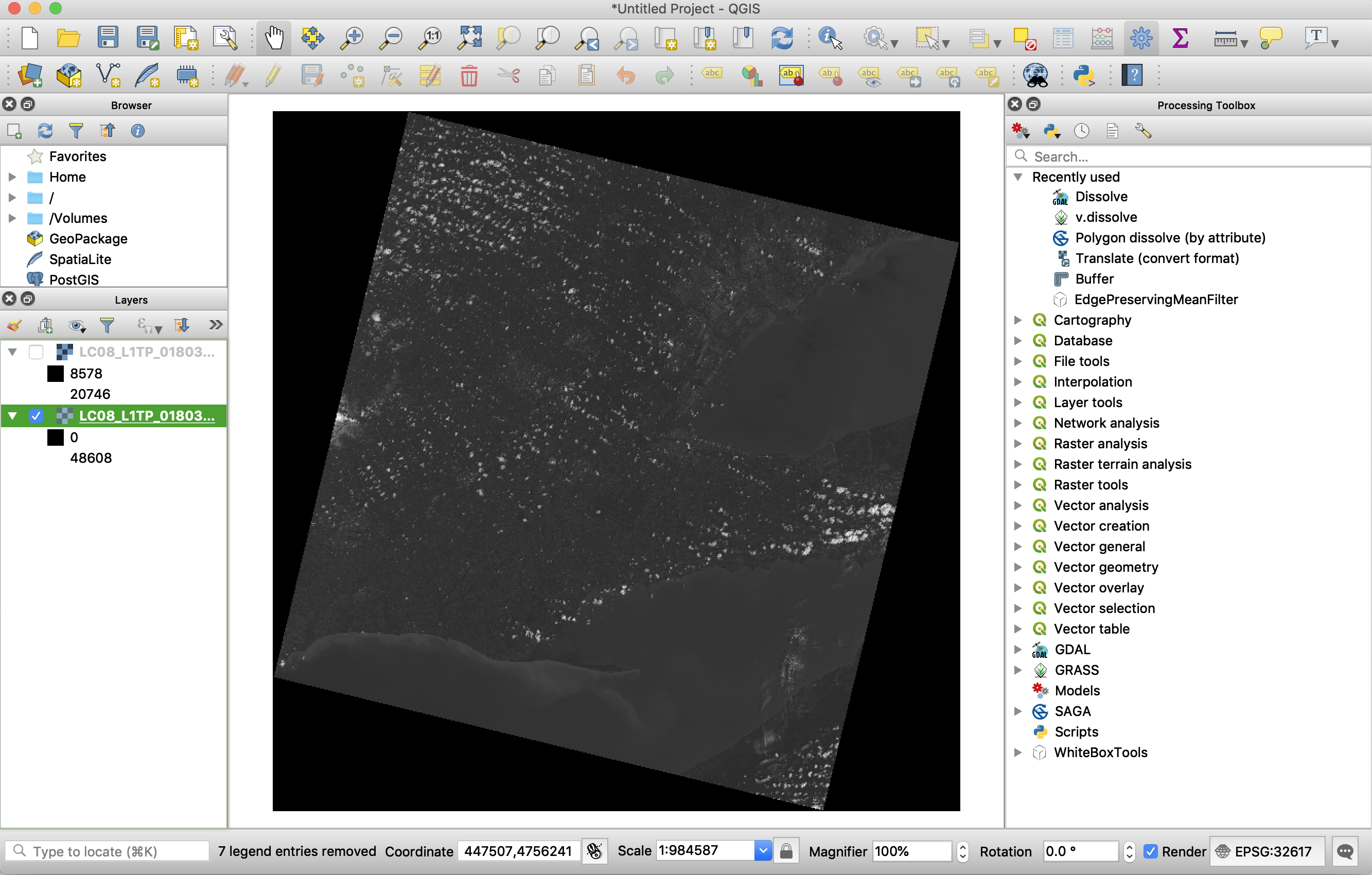
There are a couple of issues with the images as they are currently displayed. First, notice the large black triangular regions around the edges of the data. These areas are filled with a background value of zero, however, they are not being recognized as NoData values. This is partly the reason for the second issue with the displayed images, and that is the poor contrast; the areas of clouds are quite bright but all other areas have a uniformly intermediate brightness, causing very little contrast. The contrast of these two images is inadequate because the greytones used to render the images are being scaled to their minimum (those background zero values) and maximum (cloud) values. You should close the displayed images before moving on.

To solve the contrast problem, we will first set the NoData value in the images to '0', so that the minium displayed value is not taken by the background. To do this, we will use WhiteboxTool's SetNodataValue tool. We will first access WhiteboxTools using the WhiteboxTools Runner. If you haven't already done so, download the most recent version of WhiteboxTools, which includes the WhiteboxTools Runner user interface. You may launch the Runner (assuming you have Python 3 installed on your machine) by opening a command prompt (i.e. terminal application) and typing the following:

cd /path/to/whitebox_runner/script/
python3 wb_runner.py

Note: The cd command will change the working directory of your terminal. Replace /path/to/whitebox_runner/script/ with your directory path to the WhiteboxTools application. On Windows, you use \ as a path separator character and / on all other operating systems. The python3 command is used in place of the more common python command only if Python 2 is the default version of Python on your system.

You should see the following user interface displayed, after clicking the SetNodataValue menu item on the left:

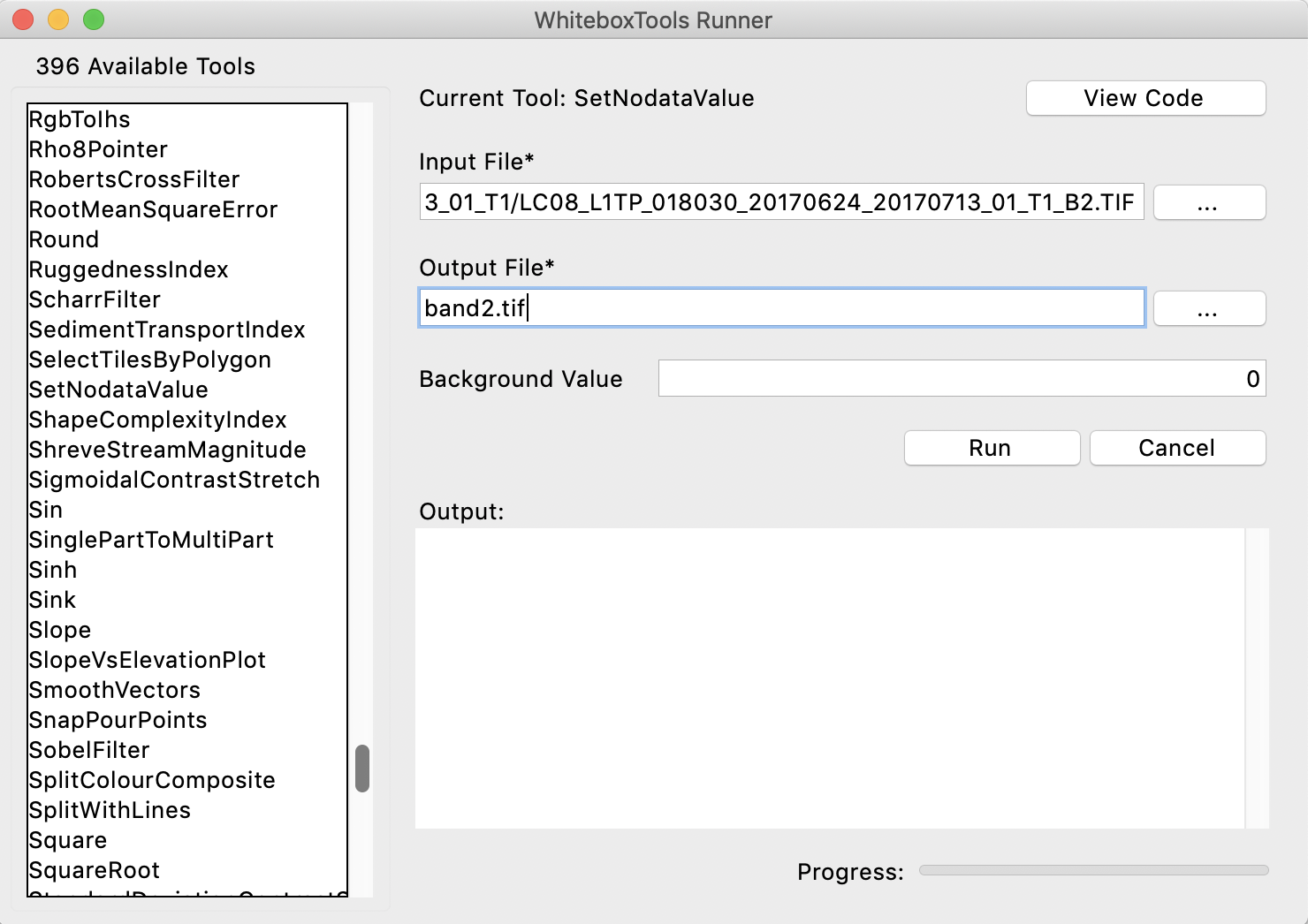
Enter LC08_L1TP_018030_20170624_20170713_01_T1_B2.TIF as the input file and call the output file band2.tif; the background value can be left to the default of 0. Press the Run button and once the application is complete, display the band2.tif image (close any open images that you currently have). You should notice that the black triangles around the edges have disappeared now.

As a caution, the images that we are using in this lab are extremely large data files and we will need substantial memory resources to process. While the computers in the undergraduate computing lab are able to handle these requirements, it is possible, if you are using your own laptop for completing this assignment, that you will run into out-of-memory errors. If this is the case, you will have no alternative but to use a computer with more memory (RAM, not hard-drive space). This will likely be the case throughout the semester as the processing of remotely sensed imagery often requires powerful workstations.

The WhiteboxTools Runner provides a very useful way of interacting with the WhiteboxTools library when we need to run a few functions but any user-interface application becomes cumbersome when we have a complex workflow or are repeating the same operation numerous times. In our case, we will need to perform the same SetNodataValue operation on all ten bands of the Landsat dataset. Doing this manually would be tedious and this is a perfect example of the type of repetitive operation that scripting is ideally suited to.

We are going to call the same SetNodataValue tool from a Python script. Your TA will provide a demonstration on how to use Python and the open-source VS Code text editor (installed on the computers in the lab) to interact with the WhiteboxTools library. For further details, please see Interfacing With Python in the WhiteboxTools user manual. NOTE: This will take some time to become comfortable with the workflow of interacting with WhiteboxTools using Python scripting (you may learn more about the Python language here). I do not expect that you will become an expert in Python programming by the end of this course; we are only hoping that you will gain a basic level of competency with using Python to interact with WhiteboxTools in this time. However, it is an essential learning outcome of this lab and will be the basis of a great deal of remote sensing applications that we will use throughout this series of lab assignments this semester.

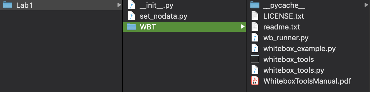
Once you are familiar with how to write Python scripts using WhiteboxTools and VS Code, create a directory named Lab1 and paste the WhiteboxTools WBT folder into this directory. Now, using VS Code, create a new file within Lab1 called __init__.py (those are two underscores preceeding and following the word init). This file will allows us to import Python modules contained within the WBT subdirectory of Lab1; the __init__.py does not need to contain anything. Now create a second script file called set_nodata.py, which will contain our code. Your directory structure should look something like the following:

Finally, paste the following code into your set_nodata.py:

from WBT.whitebox_tools import WhiteboxTools


def main():
    wbt = WhiteboxTools()
    wbt.work_dir = "/path/to/landsat/data/"

    for bandNum in range(1, 11):
        print("Working on band {}".format(bandNum))
        inFile = "LC08_L1TP_018030_20170624_20170713_01_T1_B{}.TIF".format(bandNum)
        outFile = "band{}.tif".format(bandNum)
        wbt.set_nodata_value(inFile, outFile, 0.0)

    print("All done!")


main()

Notes: Python is a space-sensitive programming language and you need to have the indentations absolutely correct in your script for it to run correctly. This is something that can often go wrong when you are copying and pasting code into a script file. Also, you will need to change the line working_dir = "/path/to/landsat/data/" to the folder containing your image data. Important if you are running this script on a computer running Microsoft Windows: Windows uses the backslash-slash (\) as the directory path separator but this is famously difficult for writing strings (i.e. text variables) containing file paths because \ is an escape character in all programming languages. To deal with this, you must represent your variables containing paths in one of the following ways:

# Uses an escaped forward character (\\)
wbt.work_dir = "\\path\\to\\landsat\\data\\"

# Uses a 'raw string' in which '\' is interpreted without escaped characters.
# Because raw strings can't end with a '\', we must use double " at the end.
wbt.work_dir = r"\path\to\landsat\data\""

# Python should also properly interpret directories using the forward
# slash on Windows.
wbt.work_dir = "/path/to/landsat/data/"

The script above first sets up the WhiteboxTools Python environment, importing the library and then setting up the working directory. The script then uses a for loop to run the SetNodataValue tool that we used previously 10 times, once for each band in the data. We use the loop iteration variable bandNum to create appropriate input and output file names associated with each of the 10 bands. It's a pretty short script, but it shows the power of being able to call remote sensing functions from a scripting language like Python. Imagine if instead of 10 multispectral bands, we were working with hundreds of bands in a hyperspectral dataset. Being able to write scripts like the one above significantly improves your competency as a remote sensing analyst.

Execute the script and allow it to complete the processing of each of the output images.

2.3. Analyze the above script and provide line-by-line description of what the script is does (10 marks; the TA will mark your answer for accuracy and clarity). For example, the line wbt = WhiteboxTools() creates an instance of a the WhiteboxTools class, which will later be used to call the set_nodata_value function. Feel free to discuss the script in groups and with your TA if there are portions of it that are unclear to you.

Now, using your data visualization software (ArcGIS, Whitebox GAT, QGIS, etc.) display the band2.tif and band6.tif images. While the NoData edges have been removed by our processing, the contrast of the images is still being affected by the very high brightness of the clouds. We will examine ways of modifying image data to improve the contrast in a later lab assignment, but for now, you can quickly improve their display by adjusting the display minimum and maximum values. In each of ArcGIS, Whitebox GAT, and QGIS this involves clipping the display min/max values in Layer Properties/Symbology tabs. Note that this does not permanently modify the image, but only the way that it is being rendered in the software.

2.4. Zoom into a grouping of the many clouds contained within the scene. Cloud cover, and particularly thick clouds, can significantly impact the usability of imagery for certain applications. Not only is the ground directly beneath clouds obscured from view, but clouds also cast shadow areas within images, which can degrade the overall image quality. Compare the appearance of clouds and areas of cloud shadows in the band 2 and band 6 images. Which of the two bands (i.e. regions of the electromagnetic spectrum) is more significantly impacted by cloud cover? Include screenshots of cloudy sections of the two images (zoomed in) to support your case. Why might there be differences in the impacts of clouds between the two images? (5 marks)

2.5. Locate Guelph Lake in the images. Guelph Lake is a relatively shallow reservoir. How does the appearance of the lake (or any waterbody for that matter) compare between the two images? What does this indicate about how the two regions of electromagnetic radiation captured by these two bands interact with water surfaces? (3 marks)

2.6. Add the panchromatic band 8 image (band8.tif) to the map and zoom into the Toronto waterfront area (you will likely need to stretch the palette for this image once displayed as well). How does the band 8 image compare to either of the other two displayed images in terms of level of detail? What is the spatial resolution of band 8 compared to the band 2? (4 marks)

2.7. The Landsat images are uncalibrated and the values that you see are simple digital numbers (DNs), which describe the relative brightness of a pixel in a unitless format. It is often necessary to calibrate images that are used for various applications (e.g. image classification) by converting the DNs to top-of-atmosphere (TOA) radiance values. This is accomplished by using multiplying each DN by a gain value and adding an offset. Read the following USGS link carefully https://landsat.usgs.gov/using-usgs-landsat-8-product, then using the band-specific information contained in the metadata file associated with the image data, provide the equations that would be used to convert bands 2, 3, and 4 (red, green, blue) of the OLI dataset into radiance values. (3 marks)

A multispectral dataset contains an enormous wealth of information, however, it can be frustrating trying to interpret these data by examining individual bands. It is possible to combine the information contained in three bands into a single colour image, known as a colour composite. Colour composites allow us to interpret the relative brightnesses, on a pixel-by-pixel basis, for three regions of the electromagnetic spectrum (i.e. bands) simultaneously. Notice that while the three bands that are represented by the composite image are being displayed using the red, green, and blue channels of your display (i.e. your monitor is creates a range of visible colours by combining each of red, green, and blue visible light in varying intensities), the bands themselves may well be derived from regions of the spectrum that fall outside of the visible light region. If, however, the three bands of a composite image correspond with the red, green, and blue bands, the resulting image will be a true colour composite and will look very much like a normal colour photograph.

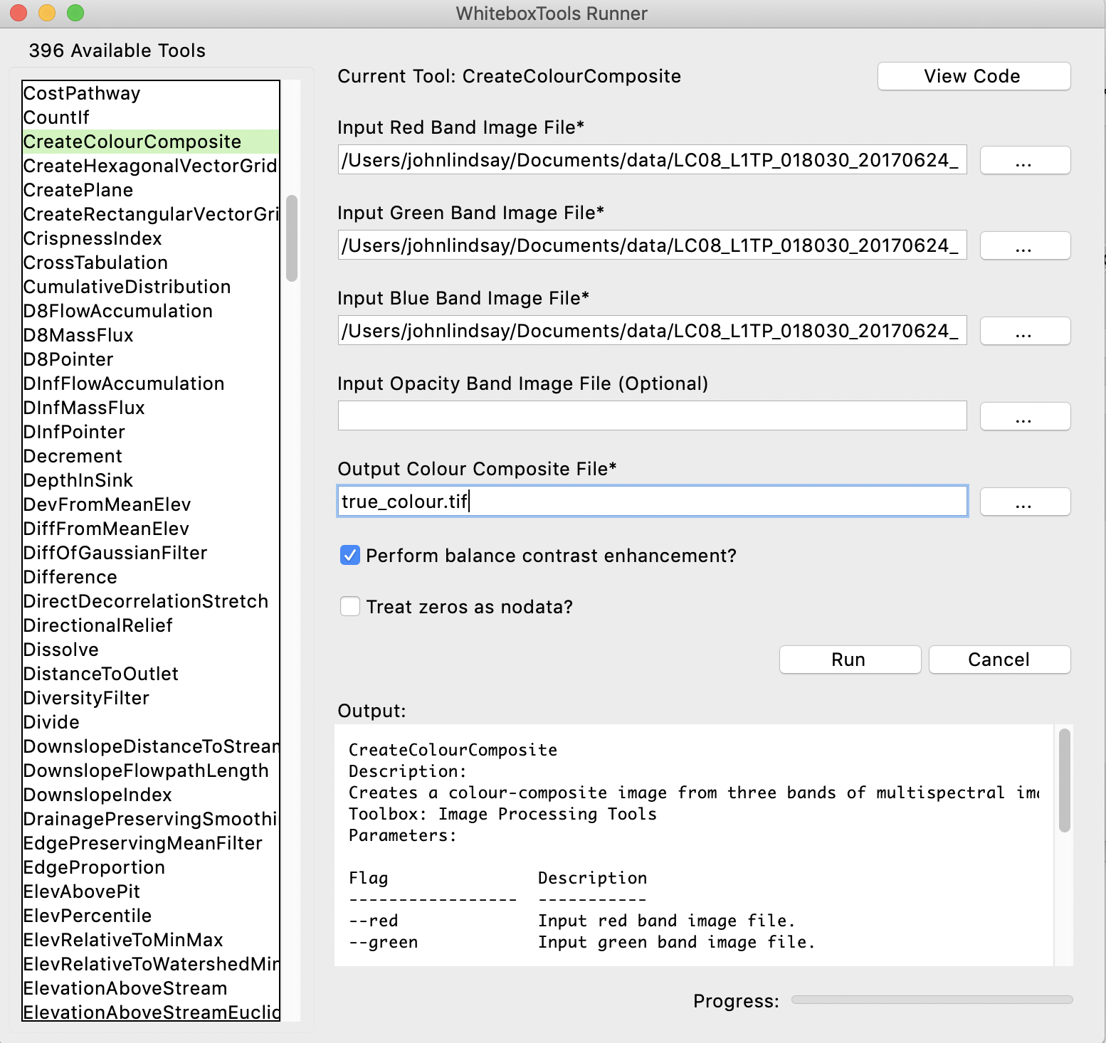
Using the CreateColourComposite tool, available from the WhiteboxTools Runner application, create a true-colour composite image (also known as a natural-colour composite). Enter band4.tif, band3.tif, and band2.tif into the red, green, and blue band image inputs and call the output file true_colour.tif. You do not need to specify an opacity image.

Using your data visualization software (ArcGIS, Whitebox GAT, QGIS, etc.), display the true_colour.tif composite image. We could refer to this image as a 4-3-2 colour composite to designate the bands that were used to create it. Include a screenshot of your true-colour composite image with your report (2 marks).

3.1. Zoom into the University of Guelph campus. What is the large bright red coloured spot, apparent in the true colour composite, and located within the Guelph campus? (1 mark)

3.2. What has caused the swirls of beige-coloured water along the shoreline of Lake Erie west of Long Point? (1 mark)

3.3. Examine the western side of Greater Toronto Area (GTA), including the Mississauga area. If you are unfamiliar with this region, use Google Maps to locate Highway 401 and Highway 407 in the colour-composite image. What causes the difference in the appearance (brightness and colour) of these two of the major east-west corridors? (1 mark)

The main benefit of multi-spectral data is that you are able to derive information about the land surface from regions of the spectrum well beyond the visible part of the spectrum. So called 'false-colour composite' images are created when bands cooresponding to one or more regions outside of the visible spectrum are placed into the red, green, blue channels of a composite colour image.

3.4. Create a 5-4-3 colour composite (i.e. place band 5 in the red channel, band 4 in the green channel, and band 3 in the blue channel) and a 7-6-4 colour composite and include print outs of these images with your hand-in. (2 marks)

3.5. Describe how each of these two 'false-colour' composite images compare to the true-colour composite image. Suggest some applications for which these images may be more appropriate than the true colour composite image. (6 marks; hint: if you Google 'Landsat band combinations', there are several useful resources, just be mindful that we are using Landsat 8 data in this lab and other Landsat satellites have different band designations.)