Image Processing Tools
- ChangeVectorAnalysis
- Closing
- CreateColourComposite
- FlipImage
- IhsToRgb
- ImageSlider
- ImageStackProfile
- IntegralImage
- LineThinning
- Mosaic
- MosaicWithFeathering
- NormalizedDifferenceIndex
- Opening
- RemoveSpurs
- Resample
- RgbToIhs
- SplitColourComposite
- ThickenRasterLine
- TophatTransform
- WriteFunctionMemoryInsertion
ChangeVectorAnalysis
Change Vector Analysis (CVA) is a change detection method that characterizes the magnitude and change direction in spectral space between two times. A change vector is the difference vector between two vectors in n-dimensional feature space defined for two observations of the same geographical location (i.e. corresponding pixels) during two dates. The CVA inputs include the set of raster images corresponding to the multispectral data for each date. Note that there must be the same number of image files (bands) for the two dates and they must be entered in the same order, i.e. if three bands, red, green, and blue are entered for date one, these same bands must be entered in the same order for date two.
CVA outputs two image files. The first image contains the change vector length, i.e. magnitude, for each pixel in the multi-spectral dataset. The second image contains information about the direction of the change event in spectral feature space, which is related to the type of change event, e.g. deforestation will likely have a different change direction than say crop growth. The vector magnitude is a continuous numerical variable. The change vector direction is presented in the form of a code, referring to the multi-dimensional sector in which the change vector occurs. A text output will be produced to provide a key describing sector codes, relating the change vector to positive or negative shifts in n-dimensional feature space.
It is common to apply a simple thresholding operation on the magnitude data to determine 'actual' change (i.e. change above some assumed level of error). The type of change (qualitatively) is then defined according to the corresponding sector code. Jensen (2015) provides a useful description of this approach to change detection.
Reference:
Jensen, J. R. (2015). Introductory Digital Image Processing: A Remote Sensing Perspective.
See Also: WriteFunctionMemoryInsertion
Parameters:
| Flag | Description |
|---|---|
| --date1 | Input raster files for the earlier date |
| --date2 | Input raster files for the later date |
| --magnitude | Output vector magnitude raster file |
| --direction | Output vector Direction raster file |
Python function:
wbt.change_vector_analysis(
    date1,
    date2,
    magnitude,
    direction,
    callback=default_callback
)
Command-line Interface:
>>./whitebox_tools -r=ChangeVectorAnalysis -v ^
--wd="/path/to/data/" ^
--date1='d1_band1.tif;d1_band2.tif;d1_band3.tif' ^
--date2='d2_band1.tif;d2_band2.tif;d2_band3.tif' ^
--magnitude=mag_out.tif --direction=dir_out.tif
Author: Dr. John Lindsay
Created: 29/04/2018
Last Modified: 29/04/2018
Closing
This tool performs a closing operation on an input greyscale image (--input). A
closing is a mathematical morphology operation involving
an erosion (minimum filter) of a dilation (maximum filter) set. Closing operations, together with the
Opening operation, is frequently used in the fields of computer vision and digital image processing for
image noise removal. The user must specify the size of the moving
window in both the x and y directions (--filterx and --filtery).
See Also: Opening, TophatTransform
Parameters:
| Flag | Description |
|---|---|
| -i, --input | Input raster file |
| -o, --output | Output raster file |
| --filterx | Size of the filter kernel in the x-direction |
| --filtery | Size of the filter kernel in the y-direction |
Python function:
wbt.closing(
    i,
    output,
    filterx=11,
    filtery=11,
    callback=default_callback
)
Command-line Interface:
>>./whitebox_tools -r=Closing -v --wd="/path/to/data/" ^
-i=image.tif -o=output.tif --filter=25
Author: Dr. John Lindsay
Created: 28/06/2017
Last Modified: 30/01/2020
CreateColourComposite
This tool can be used to create a colour-composite image from three bands of multi-spectral imagery. The user must specify the names of the input images to enter into the red, green, and blue channels of the resulting composite image. The output image uses the 32-bit aRGB colour model, and therefore, in addition to red, green and blue bands, the user may optionally specify a fourth image that will be used to determine pixel opacity (the 'a' channel). If no opacity image is specified, each pixel will be opaque. This can be useful for cropping an image to an irregular-shaped boundary. The opacity channel can also be used to create transparent gradients in the composite image.
A balance contrast enhancement (BCE) can optionally be performed on the bands prior to creation of the colour composite. While this operation will add to the runtime of CreateColourComposite, if the individual input bands have not already had contrast enhancements, then it is advisable that the BCE option be used to improve the quality of the resulting colour composite image.
NoData values in any of the input images are assigned NoData values in the output image and are not
taken into account when performing the BCE operation. Please note, not all images have NoData values
identified. When this is the case, and when the background value is 0 (often the case with
multispectral imagery), then the CreateColourComposite tool can be told to ignore zero values using
the --zeros flag.
See Also: BalanceContrastEnhancement, SplitColourComposite
Parameters:
| Flag | Description |
|---|---|
| --red | Input red band image file |
| --green | Input green band image file |
| --blue | Input blue band image file |
| --opacity | Input opacity band image file (optional) |
| -o, --output | Output colour composite file |
| --enhance | Optional flag indicating whether a balance contrast enhancement is performed |
| --zeros | Optional flag to indicate if zeros are nodata values |
Python function:
wbt.create_colour_composite(
    red,
    green,
    blue,
    output,
    opacity=None,
    enhance=True,
    zeros=False,
    callback=default_callback
)
Command-line Interface:
>>./whitebox_tools -r=CreateColourComposite -v ^
--wd="/path/to/data/" --red=band3.tif --green=band2.tif ^
--blue=band1.tif -o=output.tif
>>./whitebox_tools ^
-r=CreateColourComposite -v --wd="/path/to/data/" ^
--red=band3.tif --green=band2.tif --blue=band1.tif ^
--opacity=a.tif -o=output.tif --enhance --zeros
Author: Dr. John Lindsay
Created: 19/07/2017
Last Modified: 18/10/2019
FlipImage
This tool can be used to flip, or reflect, an image (--input) either vertically, horizontally, or both. The
axis of reflection is specified using the --direction parameter. The input image is not reflected in place;
rather, the reflected image is stored in a separate output (--output) file.
Parameters:
| Flag | Description |
|---|---|
| -i, --input | Input raster file |
| -o, --output | Output raster file |
| --direction | Direction of reflection; options include 'v' (vertical), 'h' (horizontal), and 'b' (both) |
Python function:
wbt.flip_image(
    i,
    output,
    direction="vertical",
    callback=default_callback
)
Command-line Interface:
>>./whitebox_tools -r=FlipImage -v --wd="/path/to/data/" ^
--input=in.tif -o=out.tif --direction=h
Author: Dr. John Lindsay
Created: 11/07/2017
Last Modified: 13/10/2018
IhsToRgb
This tool transforms three intensity, hue, and saturation (IHS; sometimes HSI or HIS) raster images into three equivalent multispectral images corresponding with the red, green, and blue channels of an RGB composite. Intensity refers to the brightness of a color, hue is related to the dominant wavelength of light and is perceived as color, and saturation is the purity of the color (Koutsias et al., 2000). There are numerous algorithms for performing a red-green-blue (RGB) to IHS transformation. This tool uses the transformation described by Haydn (1982). Note that, based on this transformation, the input IHS values must follow the ranges:
0 < I < 1
0 < H < 2PI
0 < S < 1
The output red, green, and blue images will have values ranging from 0 to 255. The user must specify the names of the
intensity, hue, and saturation images (--intensity, --hue, --saturation). These images will generally be created using
the RgbToIhs tool. The user must also specify the names of the output red, green, and blue images (--red, --green,
--blue). Image enhancements, such as contrast stretching, are often performed on the individual IHS components, which are
then inverse transformed back in RGB components using this tool. The output RGB components can then be used to create an
improved color composite image.
References:
Haydn, R., Dalke, G.W. and Henkel, J. (1982) Application of the IHS color transform to the processing of multisensor data and image enhancement. Proc. of the Inter- national Symposium on Remote Sensing of Arid and Semiarid Lands, Cairo, 599-616.
Koutsias, N., Karteris, M., and Chuvico, E. (2000). The use of intensity-hue-saturation transformation of Landsat-5 Thematic Mapper data for burned land mapping. Photogrammetric Engineering and Remote Sensing, 66(7), 829-840.
See Also: RgbToIhs, BalanceContrastEnhancement, DirectDecorrelationStretch
Parameters:
| Flag | Description |
|---|---|
| --intensity | Input intensity file |
| --hue | Input hue file |
| --saturation | Input saturation file |
| --red | Output red band file. Optionally specified if colour-composite not specified |
| --green | Output green band file. Optionally specified if colour-composite not specified |
| --blue | Output blue band file. Optionally specified if colour-composite not specified |
| -o, --output | Output colour-composite file. Only used if individual bands are not specified |
Python function:
wbt.ihs_to_rgb(
    intensity,
    hue,
    saturation,
    red=None,
    green=None,
    blue=None,
    output=None,
    callback=default_callback
)
Command-line Interface:
>>./whitebox_tools -r=IhsToRgb -v --wd="/path/to/data/" ^
--intensity=intensity.tif --hue=hue.tif ^
--saturation=saturation.tif --red=band3.tif --green=band2.tif ^
--blue=band1.tif
>>./whitebox_tools -r=IhsToRgb -v ^
--wd="/path/to/data/" --intensity=intensity.tif --hue=hue.tif ^
--saturation=saturation.tif --composite=image.tif
Author: Dr. John Lindsay
Created: 25/07/2017
Last Modified: 22/10/2019
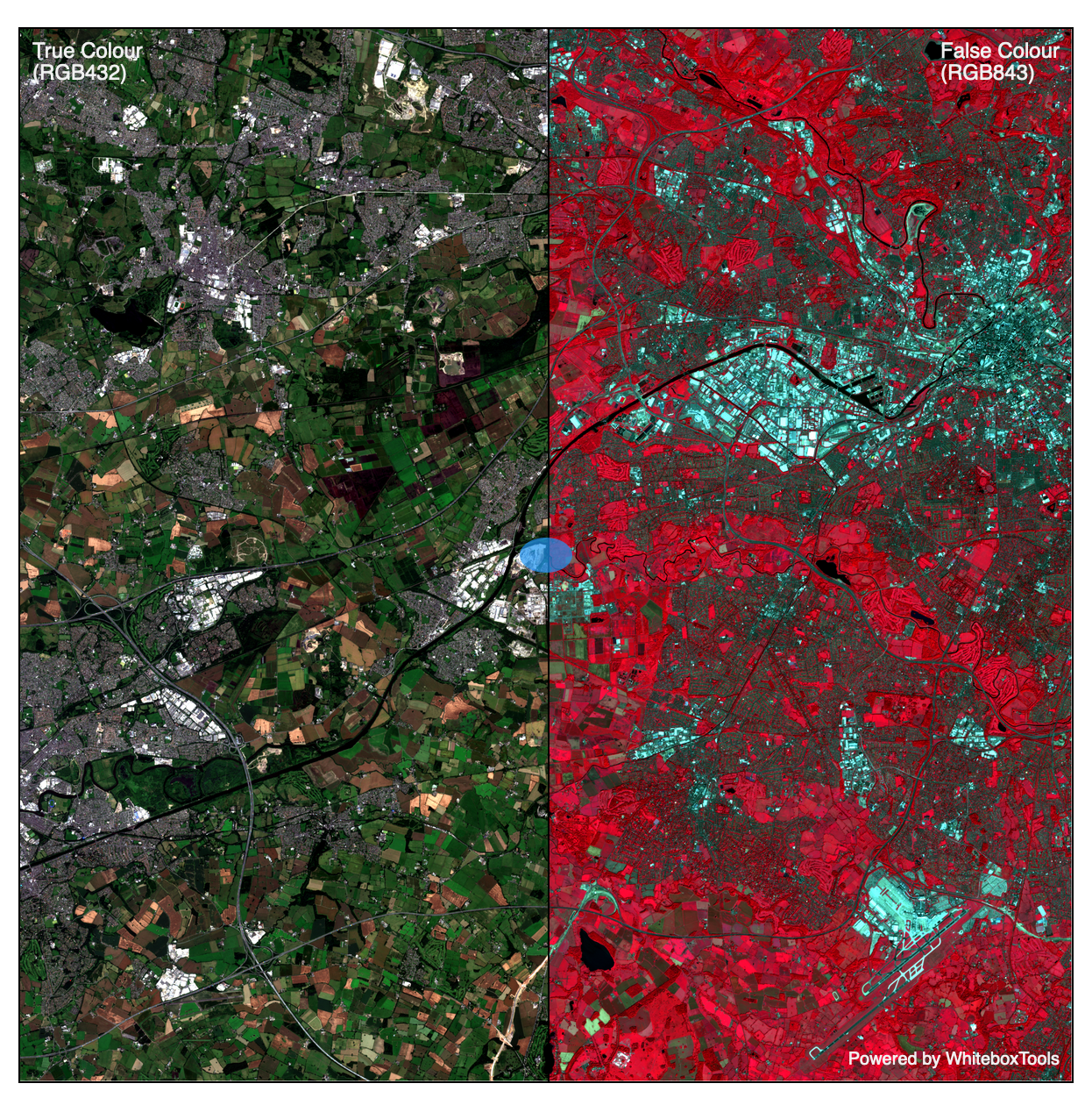
ImageSlider
Note this tool is part of a WhiteboxTools extension toolset. Please contact Whitebox Geospatial Inc. for information about purchasing a license activation key (https://www.whiteboxgeo.com).
This tool creates an interactive image slider from two input images (--input1 and --input2). An
image slider is an interactive visualization of two overlapping images, in which the user moves the
position of a slider bar to hide or reveal one of the overlapping images. The output (--output)
is an HTML file. Each of the two input images may be rendered in one of several available palettes.
If the input image is a colour composite image, no palette is required. Labels may also be optionally
associated with each of the images, displayed in the upper left and right corners. The user must also
specify the image height (--height) in the output file. Note that the output is simply HTML, CSS, and
javascript code, which can be readily embedded in other documents.
The following is an example of what the output of this tool looks like. Click the image for an interactive example.
Parameters:
| Flag | Description |
|---|---|
| --i1, --input1 | Name of the left input image file |
| --p1, --palette1 | Left image palette; options are 'grey', 'atlas', 'high_relief', 'arid', 'soft', 'muted', 'purple', 'viridi', 'gn_yl', 'pi_y_g', 'bl_yl_rd', 'deep', and 'rgb' |
| --r1, --reverse1 | Reverse left image palette? |
| --l1, --label1 | Left image label (leave blank for none) |
| --i2, --input2 | Name of the right input image file |
| --p2, --palette2 | Right image palette; options are 'grey', 'atlas', 'high_relief', 'arid', 'soft', 'muted', 'purple', 'viridi', 'gn_yl', 'pi_y_g', 'bl_yl_rd', 'deep', and 'rgb' |
| --r2, --reverse2 | Reverse right image palette? |
| --l2, --label2 | Right image label (leave blank for none) |
| -o, --output | Name of the output HTML file (*.html) |
| -h, --height | Image height, in pixels |
Python function:
wbt.image_slider(
    input1,
    input2,
    output,
    palette1="grey",
    reverse1=False,
    label1="",
    palette2="grey",
    reverse2=False,
    label2="",
    height=600,
    callback=default_callback
)
Command-line Interface:
>> ./whitebox_tools -r=ImageSlider --i1=band1.tif --p1=soft ^
--r1=false --l1="Label 1" --i2=band2.tif --p1=soft --r2=false ^
--l2="Label 2" -o=class_properties.html
Source code is unavailable due to proprietary license.
Author: Whitebox Geospatial Inc. (c)
Created: 29/04/2021
Last Modified: 29/04/2021
ImageStackProfile
This tool can be used to plot an image stack profile (i.e. a signature) for a set of points (--points) and
a multispectral image stack (--inputs). The tool outputs an interactive SVG line graph embedded in an
HTML document (--output). If the input points vector contains multiple points, each input point will
be associated with a single line in the output plot. The order of vertices in each signature line is
determined by the order of images specified in the --inputs parameter. At least two input images are
required to run this operation. Note that this tool does not require multispectral images as
inputs; other types of data may also be used as the image stack. Also note that the input images should be
single-band, continuous greytone rasters. RGB colour images are not good candidates for this tool.
If you require the raster values to be saved in the vector points file's attribute table, or if you need the raster values to be output as text, you may use the ExtractRasterValuesAtPoints tool instead.
See Also: ExtractRasterValuesAtPoints
Parameters:
| Flag | Description |
|---|---|
| -i, --inputs | Input multispectral image files |
| --points | Input vector points file |
| -o, --output | Output HTML file |
Python function:
wbt.image_stack_profile(
    inputs,
    points,
    output,
    callback=default_callback
)
Command-line Interface:
>>./whitebox_tools -r=ImageStackProfile -v ^
--wd="/path/to/data/" -i='image1.tif;image2.tif;image3.tif' ^
--points=pts.shp -o=output.html
Author: Dr. John Lindsay
Created: 15/03/2018
Last Modified: 13/10/2018
IntegralImage
This tool transforms an input raster image into an integral image, or summed area table. Integral images are the two-dimensional equivalent to a cumulative distribution function. Each pixel contains the sum of all pixels contained within the enclosing rectangle above and to the left of a pixel. Images with a very large number of grid cells will likely experience numerical overflow errors when converted to an integral image. Integral images are used in a wide variety of computer vision and digital image processing applications, including texture mapping. They allow for the efficient calculation of very large filters and are the basis of several of WhiteboxTools's image filters.
Reference:
Crow, F. C. (1984, January). Summed-area tables for texture mapping. In ACM SIGGRAPH computer graphics (Vol. 18, No. 3, pp. 207-212). ACM.
Parameters:
| Flag | Description |
|---|---|
| -i, --input | Input raster file |
| -o, --output | Output raster file |
Python function:
wbt.integral_image(
    i,
    output,
    callback=default_callback
)
Command-line Interface:
>>./whitebox_tools -r=IntegralImage -v --wd="/path/to/data/" ^
-i=image.tif -o=output.tif
Author: Dr. John Lindsay
Created: 26/06/2017
Last Modified: 13/10/2018
LineThinning
This image processing tool reduces all polygons in a Boolean raster image to their single-cell wide skeletons. This operation is sometimes called line thinning or skeletonization. In fact, the input image need not be truly Boolean (i.e. contain only 1's and 0's). All non-zero, positive values are considered to be foreground pixels while all zero valued cells are considered background pixels. The RemoveSpurs tool is useful for cleaning up an image before performing a line thinning operation.
Note: Unlike other filter-based operations in WhiteboxTools, this algorithm can't easily be parallelized because the output raster must be read and written to during the same loop.
See Also: RemoveSpurs, ThickenRasterLine
Parameters:
| Flag | Description |
|---|---|
| -i, --input | Input raster file |
| -o, --output | Output raster file |
Python function:
wbt.line_thinning(
    i,
    output,
    callback=default_callback
)
Command-line Interface:
>>./whitebox_tools -r=LineThinning -v --wd="/path/to/data/" ^
--input=DEM.tif -o=output.tif
Author: Dr. John Lindsay
Created: 05/07/2017
Last Modified: 16/02/2019
Mosaic
This tool will create an image mosaic from one or more input image files using one of three resampling methods including, nearest neighbour, bilinear interpolation, and cubic convolution. The order of the input source image files is important. Grid cells in the output image will be assigned the corresponding value determined from the last image found in the list to possess an overlapping coordinate.
Note that when the --inputs parameter is left unspecified, the tool will use
all of the .tif, .tiff, .rdc, .flt, .sdat, and .dep files located in the working directory.
This can be a useful way of mosaicing large number of tiles, particularly when
the text string that would be required to specify all of the input tiles is
longer than the allowable limit.
This is the preferred mosaicing tool to use when appending multiple images with little to no overlapping areas, e.g. tiled data. When images have significant overlap areas, users are advised to use the MosaicWithFeathering tool instead.
Resample is very similar in operation to the Mosaic tool. The Resample tool should be used when there is an existing image into which you would like to dump information from one or more source images. If the source images are more extensive than the destination image, i.e. there are areas that extend beyond the destination image boundaries, these areas will not be represented in the updated image. Grid cells in the destination image that are not overlapping with any of the input source images will not be updated, i.e. they will possess the same value as before the resampling operation. The Mosaic tool is used when there is no existing destination image. In this case, a new image is created that represents the bounding rectangle of each of the two or more input images. Grid cells in the output image that do not overlap with any of the input images will be assigned the NoData value.
See Also: MosaicWithFeathering
Parameters:
| Flag | Description |
|---|---|
| -i, --inputs | Input raster files |
| -o, --output | Output raster file |
| --method | Resampling method; options include 'nn' (nearest neighbour), 'bilinear', and 'cc' (cubic convolution) |
Python function:
wbt.mosaic(
    output,
    inputs=None,
    method="nn",
    callback=default_callback
)
Command-line Interface:
>>./whitebox_tools -r=Mosaic -v --wd='/path/to/data/' ^
-i='image1.tif;image2.tif;image3.tif' -o=dest.tif ^
--method='cc'
Author: Dr. John Lindsay
Created: 02/01/2018
Last Modified: 03/09/2020
MosaicWithFeathering
This tool will create a mosaic from two input images. It is similar in operation to the Mosaic tool, however, this tool is the preferred method of mosaicing images when there is significant overlap between the images. For areas of overlap, the feathering method will calculate the output value as a weighted combination of the two input values, where the weights are derived from the squared distance of the pixel to the edge of the data in each of the input raster files. Therefore, less weight is assigned to an image's pixel value where the pixel is very near the edge of the image. Note that the distance is actually calculated to the edge of the grid and not necessarily the edge of the data, which can differ if the image has been rotated during registration. The result of this feathering method is that the output mosaic image should have very little evidence of the original image edges within the overlapping area.
Unlike the Mosaic tool, which can take multiple input images, this tool only accepts two input images. Mosaic is therefore useful when there are many, adjacent or only slightly overlapping images, e.g. for tiled data sets.
Users may want to use the HistogramMatching tool prior to mosaicing if the two input images differ significantly in their radiometric properties. i.e. if image contrast differences exist.
See Also: Mosaic, HistogramMatching
Parameters:
| Flag | Description |
|---|---|
| --i1, --input1 | Input raster file to modify |
| --i2, --input2 | Input reference raster file |
| -o, --output | Output raster file |
| --method | Resampling method; options include 'nn' (nearest neighbour), 'bilinear', and 'cc' (cubic convolution) |
| --weight |
Python function:
wbt.mosaic_with_feathering(
    input1,
    input2,
    output,
    method="cc",
    weight=4.0,
    callback=default_callback
)
Command-line Interface:
>>./whitebox_tools -r=MosaicWithFeathering -v ^
--wd='/path/to/data/' --input1='image1.tif' ^
--input2='image2.tif' -o='output.tif' --method='cc' ^
--weight=4.0
Author: Dr. John Lindsay
Created: 29/12/2018
Last Modified: 02/01/2019
NormalizedDifferenceIndex
This tool can be used to calculate a normalized difference index (NDI) from two bands of multispectral image data.
A NDI of two band images (image1 and image2) takes the general form:
NDI = (image1 - image2) / (image1 + image2 + c)
Where c is a correction factor sometimes used to avoid division by zero. It is, however, often set to 0.0. In fact,
the NormalizedDifferenceIndex tool will set all pixels where image1 + image2 = 0 to 0.0 in the output image. While
this is not strictly mathematically correct (0 / 0 = infinity), it is often the intended output in these cases.
NDIs generally takes the value range -1.0 to 1.0, although in practice the range of values for a particular image scene may be more restricted than this.
NDIs have two important properties that make them particularly useful for remote sensing applications. First, they emphasize certain aspects of the shape of the spectral signatures of different land covers. Secondly, they can be used to de-emphasize the effects of variable illumination within a scene. NDIs are therefore frequently used in the field of remote sensing to create vegetation indices and other indices for emphasizing various land-covers and as inputs to analytical operations like image classification. For example, the normalized difference vegetation index (NDVI), one of the most common image-derived products in remote sensing, is calculated as:
NDVI = (NIR - RED) / (NIR + RED)
The optimal soil adjusted vegetation index (OSAVI) is:
OSAVI = (NIR - RED) / (NIR + RED + 0.16)
The normalized difference water index (NDWI), or normalized difference moisture index (NDMI), is:
NDWI = (NIR - SWIR) / (NIR + SWIR)
The normalized burn ratio 1 (NBR1) and normalized burn ration 2 (NBR2) are:
NBR1 = (NIR - SWIR2) / (NIR + SWIR2)
NBR2 = (SWIR1 - SWIR2) / (SWIR1 + SWIR2)
In addition to NDIs, Simple Ratios of image bands, are also commonly used as inputs to other remote sensing applications like image classification. Simple ratios can be calculated using the Divide tool. Division by zero, in this case, will result in an output NoData value.
See Also: Divide
Parameters:
| Flag | Description |
|---|---|
| --input1 | Input image 1 (e.g. near-infrared band) |
| --input2 | Input image 2 (e.g. red band) |
| -o, --output | Output raster file |
| --clip | Optional amount to clip the distribution tails by, in percent |
| --correction | Optional adjustment value (e.g. 1, or 0.16 for the optimal soil adjusted vegetation index, OSAVI) |
Python function:
wbt.normalized_difference_index(
    input1,
    input2,
    output,
    clip=0.0,
    correction=0.0,
    callback=default_callback
)
Command-line Interface:
>>./whitebox_tools -r=NormalizedDifferenceIndex -v ^
--wd="/path/to/data/" --input1=band4.tif --input2=band3.tif ^
-o=output.tif
>>./whitebox_tools -r=NormalizedDifferenceIndex ^
-v --wd="/path/to/data/" --input1=band4.tif --input2=band3.tif ^
-o=output.tif --clip=1.0 --adjustment=0.16
Author: Dr. John Lindsay
Created: 26/06/2017
Last Modified: 24/02/2019
Opening
This tool performs an opening operation on an input greyscale image (--input). An
opening is a mathematical morphology operation involving
a dilation (maximum filter) on an erosion (minimum filter) set. Opening operations, together with the
Closing operation, is frequently used in the fields of computer vision and digital image processing for
image noise removal. The user must specify the size of the moving window in both the x and y directions
(--filterx and --filtery).
See Also: Closing, TophatTransform
Parameters:
| Flag | Description |
|---|---|
| -i, --input | Input raster file |
| -o, --output | Output raster file |
| --filterx | Size of the filter kernel in the x-direction |
| --filtery | Size of the filter kernel in the y-direction |
Python function:
wbt.opening(
    i,
    output,
    filterx=11,
    filtery=11,
    callback=default_callback
)
Command-line Interface:
>>./whitebox_tools -r=Opening -v --wd="/path/to/data/" ^
-i=image.tif -o=output.tif --filter=25
Author: Dr. John Lindsay
Created: 28/06/2017
Last Modified: 30/01/2020
RemoveSpurs
This image processing tool removes small irregularities (i.e. spurs) on the boundaries of objects in a
Boolean input raster image (--input). This operation is sometimes called pruning. Remove Spurs is a useful tool
for cleaning an image before performing a line thinning operation. In fact, the input image need not be truly
Boolean (i.e. contain only 1's and 0's). All non-zero, positive values are considered to be foreground pixels
while all zero valued cells are considered background pixels.
Note: Unlike other filter-based operations in WhiteboxTools, this algorithm can't easily be parallelized because the output raster must be read and written to during the same loop.
See Also: LineThinning
Parameters:
| Flag | Description |
|---|---|
| -i, --input | Input raster file |
| -o, --output | Output raster file |
| --iterations | Maximum number of iterations |
Python function:
wbt.remove_spurs(
    i,
    output,
    iterations=10,
    callback=default_callback
)
Command-line Interface:
>>./whitebox_tools -r=RemoveSpurs -v --wd="/path/to/data/" ^
--input=DEM.tif -o=output.tif --iterations=10
Author: Dr. John Lindsay
Created: 05/07/2017
Last Modified: 16/02/2019
Resample
This tool can be used to modify the grid resolution of one or more rasters. The user
specifies the names of one or more input rasters (--inputs) and the output raster
(--output). The resolution of the output raster is determined either using a
specified --cell_size parameter, in which case the output extent is determined by the
combined extent of the inputs, or by an optional base raster (--base), in which case
the output raster spatial extent matches that of the base file. This operation is similar
to the Mosaic tool, except that Resample modifies the output resolution. The Resample
tool may also be used with a single input raster (when the user wants to modify its
spatial resolution, whereas, Mosaic always includes multiple inputs.
If the input source images are more extensive than the base image (if optionally specified), these areas will not be represented in the output image. Grid cells in the output image that are not overlapping with any of the input source images will not be assigned the NoData value, which will be the same as the first input image. Grid cells in the output image that overlap with multiple input raster cells will be assigned the last input value in the stack. Thus, the order of input images is important.
See Also: Mosaic
Parameters:
| Flag | Description |
|---|---|
| -i, --inputs | Input raster files |
| -o, --output | Output raster file |
| --cell_size | Optionally specified cell size of output raster. Not used when base raster is specified |
| --base | Optionally specified input base raster file. Not used when a cell size is specified |
| --method | Resampling method; options include 'nn' (nearest neighbour), 'bilinear', and 'cc' (cubic convolution) |
Python function:
wbt.resample(
    inputs,
    output,
    cell_size=None,
    base=None,
    method="cc",
    callback=default_callback
)
Command-line Interface:
>>./whitebox_tools -r=Resample -v --wd='/path/to/data/' ^
-i='image1.tif;image2.tif;image3.tif' --destination=dest.tif ^
--method='cc
Author: Dr. John Lindsay
Created: 01/01/2018
Last Modified: 25/08/2020
RgbToIhs
This tool transforms three raster images of multispectral data (red, green, and blue channels) into their equivalent intensity, hue, and saturation (IHS; sometimes HSI or HIS) images. Intensity refers to the brightness of a color, hue is related to the dominant wavelength of light and is perceived as color, and saturation is the purity of the color (Koutsias et al., 2000). There are numerous algorithms for performing a red-green-blue (RGB) to IHS transformation. This tool uses the transformation described by Haydn (1982). Note that, based on this transformation, the output IHS values follow the ranges:
0 < I < 1
0 < H < 2PI
0 < S < 1
The user must specify the names of the red, green, and blue images (--red, --green, --blue). Importantly, these
images need not necessarily correspond with the specific regions of the electromagnetic spectrum that are red, green,
and blue. Rather, the input images are three multispectral images that could be used to create a RGB color composite.
The user must also specify the names of the output intensity, hue, and saturation images (--intensity, --hue,
--saturation). Image enhancements, such as contrast stretching, are often performed on the IHS components, which are
then inverse transformed back in RGB components to then create an improved color composite image.
References:
Haydn, R., Dalke, G.W. and Henkel, J. (1982) Application of the IHS color transform to the processing of multisensor data and image enhancement. Proc. of the Inter- national Symposium on Remote Sensing of Arid and Semiarid Lands, Cairo, 599-616.
Koutsias, N., Karteris, M., and Chuvico, E. (2000). The use of intensity-hue-saturation transformation of Landsat-5 Thematic Mapper data for burned land mapping. Photogrammetric Engineering and Remote Sensing, 66(7), 829-840.
See Also: IhsToRgb, BalanceContrastEnhancement, DirectDecorrelationStretch
Parameters:
| Flag | Description |
|---|---|
| --red | Input red band image file. Optionally specified if colour-composite not specified |
| --green | Input green band image file. Optionally specified if colour-composite not specified |
| --blue | Input blue band image file. Optionally specified if colour-composite not specified |
| --composite | Input colour-composite image file. Only used if individual bands are not specified |
| --intensity | Output intensity raster file |
| --hue | Output hue raster file |
| --saturation | Output saturation raster file |
Python function:
wbt.rgb_to_ihs(
    intensity,
    hue,
    saturation,
    red=None,
    green=None,
    blue=None,
    composite=None,
    callback=default_callback
)
Command-line Interface:
>>./whitebox_tools -r=RgbToIhs -v --wd="/path/to/data/" ^
--red=band3.tif --green=band2.tif --blue=band1.tif ^
--intensity=intensity.tif --hue=hue.tif ^
--saturation=saturation.tif
>>./whitebox_tools -r=RgbToIhs -v ^
--wd="/path/to/data/" --composite=image.tif ^
--intensity=intensity.tif --hue=hue.tif ^
--saturation=saturation.tif
Author: Dr. John Lindsay
Created: 25/07/2017
Last Modified: 22/10/2019
SplitColourComposite
This tool can be used to split a red-green-blue (RGB) colour-composite image into three separate bands of
multi-spectral imagery. The user must specify the input image (--input) and output red, green, blue images
(--red, --green, --blue).
See Also: CreateColourComposite
Parameters:
| Flag | Description |
|---|---|
| -i, --input | Input colour composite image file |
| --red | Output red band file |
| --green | Output green band file |
| --blue | Output blue band file |
Python function:
wbt.split_colour_composite(
    i,
    red=None,
    green=None,
    blue=None,
    callback=default_callback
)
Command-line Interface:
>>./whitebox_tools -r=SplitColourComposite -v ^
--wd="/path/to/data/" -i=input.tif --red=red.tif ^
--green=green.tif --blue=blue.tif
Author: Dr. John Lindsay
Created: 15/07/2017
Last Modified: 12/04/2019
ThickenRasterLine
This image processing tool can be used to thicken single-cell wide lines within a raster file along diagonal sections of the lines. Because of the limitation of the raster data format, single-cell wide raster lines can be traversed along diaganol sections without passing through a line grid cell. This causes problems for various raster analysis functions for which lines are intended to be barriers. This tool will thicken raster lines, such that it is impossible to cross a line without passing through a line grid cell. While this can also be achieved using a maximum filter, unlike the filter approach, this tool will result in the smallest possible thickening to achieve the desired result.
All non-zero, positive values are considered to be foreground pixels while all zero valued cells or NoData cells are considered background pixels.
Note: Unlike other filter-based operations in WhiteboxTools, this algorithm can't easily be parallelized because the output raster must be read and written to during the same loop.
See Also: LineThinning
Parameters:
| Flag | Description |
|---|---|
| -i, --input | Input raster file |
| -o, --output | Output raster file |
Python function:
wbt.thicken_raster_line(
    i,
    output,
    callback=default_callback
)
Command-line Interface:
>>./whitebox_tools -r=ThickenRasterLine -v ^
--wd="/path/to/data/" --input=DEM.tif -o=output.tif
Author: Dr. John Lindsay
Created: 04/07/2017
Last Modified: 13/10/2018
TophatTransform
This tool performs either a white or black top-hat transform
on an input image. A top-hat transform is a common digital image processing operation used for various tasks, such
as feature extraction, background equalization, and image enhancement. The size of the rectangular structuring element
used in the filtering can be specified using the --filterx and --filtery flags.
There are two distinct types of top-hat transform including white and black top-hat transforms. The white top-hat
transform is defined as the difference between the input image and its opening
by some structuring element. An opening operation is the dilation
(maximum filter) of an erosion (minimum filter) image.
The black top-hat transform, by comparison, is defined as the difference between the
closing and the input image. The user specifies which of the two
flavours of top-hat transform the tool should perform by specifying either 'white' or 'black' with the --variant flag.
See Also: Closing, Opening, MaximumFilter, MinimumFilter
Parameters:
| Flag | Description |
|---|---|
| -i, --input | Input raster file |
| -o, --output | Output raster file |
| --filterx | Size of the filter kernel in the x-direction |
| --filtery | Size of the filter kernel in the y-direction |
| --variant | Optional variant value. Options include 'white' and 'black' |
Python function:
wbt.tophat_transform(
    i,
    output,
    filterx=11,
    filtery=11,
    variant="white",
    callback=default_callback
)
Command-line Interface:
>>./whitebox_tools -r=TophatTransform -v ^
--wd="/path/to/data/" -i=image.tif -o=output.tif --filter=25
Author: Dr. John Lindsay
Created: 28/06/2017
Last Modified: 30/01/2020
WriteFunctionMemoryInsertion
Jensen (2015) describes write function memory (WFM) insertion as a simple yet effective method of visualizing land-cover change between two or three dates. WFM insertion may be used to qualitatively inspect change in any type of registered, multi-date imagery. The technique operates by creating a red-green-blue (RGB) colour composite image based on co-registered imagery from two or three dates. If two dates are input, the first date image will be put into the red channel, while the second date image will be put into both the green and blue channels. The result is an image where the areas of change are displayed as red (date 1 is brighter than date 2) and cyan (date 1 is darker than date 2), and areas of little change are represented in grey-tones. The larger the change in pixel brightness between dates, the more intense the resulting colour will be.
If images from three dates are input, the resulting composite can contain many distinct colours. Again, more intense the colours are indicative of areas of greater land-cover change among the dates, while areas of little change are represented in grey-tones. Interpreting the direction of change is more difficult when three dates are used. Note that for multi-spectral imagery, only one band from each date can be used for creating a WFM insertion image.
Reference:
Jensen, J. R. (2015). Introductory Digital Image Processing: A Remote Sensing Perspective.
See Also: CreateColourComposite, ChangeVectorAnalysis
Parameters:
| Flag | Description |
|---|---|
| --i1, --input1 | Input raster file associated with the first date |
| --i2, --input2 | Input raster file associated with the second date |
| --i3, --input3 | Optional input raster file associated with the third date |
| -o, --output | Output raster file |
Python function:
wbt.write_function_memory_insertion(
    input1,
    input2,
    output,
    input3=None,
    callback=default_callback
)
Command-line Interface:
>>./whitebox_tools -r=WriteFunctionMemoryInsertion -v ^
--wd="/path/to/data/" -i1=input1.tif -i2=input2.tif ^
-o=output.tif
Author: Dr. John Lindsay
Created: 18/07/2017
Last Modified: 13/10/2018